Using the Spotify Algorithm to Find High Energy Physics Particles

Few steps, python guide to particle tracking with Approximate Nearest Neighbor library Annoy.

Neighboring particle hits collected in “buckets”

For a refresher on processing and visualizing particles with Python, check out my earlier post. Tracking particles in High Energy Physics is about connecting together the hits produced by the same particle. In a typical High Luminosity collision event, 100K hits are produced by 10K particles leading to an average particle size of 10 hits.

The challenge is then to connect the right 10 hits together from a collection of similarly looking 100K hits and to do it under a second! This is the reason why we turn to “outside-the-box” solutions and typically ones that are used to process massive datasets. What about several millions songs datasets?

Spotify is the indisputable winner when it comes to suggestions of songs you might like next. The computational trick here is to search for similarities between songs in a very large database and Spotify’s Annoy library does so elegantly. It is open-source, simple to use and available in several languages. Let’s see how to use it to find light-speed particles.

Annoy can be quickly installed with pip

#Version used in this guide :  1.17.0
pip install annoy

The general idea behind Approximate Nearest Neighbor techniques is to return approximately and quickly the set of points closest to a query point. The first step is to build an index of the dataset while specifying the metric used to asses the similarity between points. Then, when a query is made (x4 in the figure), the set of similar points is retrieved using approximate techniques rather than an exhaustive search. Annoy uses random projection to quickly bin the data and this makes the search very fast.

If you haven’t guessed it yet, our neighbors in particle tracking will be the hits produced by the same particle. Different queries on the dataset will produce different sets of neighbors and our goal is find a least a particle in each set. The collision event we will use is again from the public TrackML dataset.

To build an index using Annoy, we only need to specify the number of features per hit and the similarity metric. As a first step, we will only the 3D coordinates of the hits with an angular distance. The angular distance ensures that the neighboring hits are aligned with respect to the origin. As will be shown later, this is a very good starting criteria. Let’s then, write a function that builds an index and fills it with data.

from annoy import AnnoyIndex
def buildAnnoyIndex(data,metric="angular",ntrees=5):
    f = data.shape[1]
    idx = AnnoyIndex(f,metric)  
    for i,d in enumerate(data):
        idx.add_item(i, d)
    idx.build(ntrees) 
    return idx

To ensure a higher accuracy, multiple random projections are built through the parameter “ntrees”. To ensure a faster search, we use only 5 trees.

Building an ANN index on a collision event is done with the following lines:

import pandas as pd
data=pd.read_csv("lhc_event.csv")
annoy_idx=buildAnnoyIndex(data[["x","y","z"]].values)

Now that the dataset is stored in the “annoy_idx” variable, we are able to perform queries. The function that allows to return the approximate nearest neighbors of a query hit is the following:

annoy_idx.get_nns_by_item(hit_id,Nb_neighbors)

The query hit is specified through its index in the dataset and the Nb_neighbors indicates the number of closest hits to return. This function then returns the indices of the approximate neighbors. It is also possible to return the distance value by turning on the option parameter include_distances=True

When setting the Nb_neighbors to 20 and selecting randomly a hit index, we get the following result:

hit_id=467
Nb_neighbors=20
annoy_idx.get_nns_by_item(hit_id,Nb_neighbors)
Out : [467, 468, 469, 470, 471, 474, 466, 472, 473, 476, 475, 477, 478, 480, 465, 479, 18519, 18521, 495, 18520]

We can see the hits associated to these “bucket” indices as follows:

bucket_idx=annoy_idx.get_nns_by_item(hit_id,Nb_neighbors)
data.iloc[bucket_idx]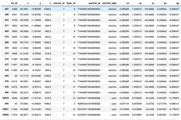

Turns out our random query hit is a lucky electron! Notice that the index column of the dataframe is exactly our ANN bucket. We can also see that the hits following our query seem the share the same particle_id=774646073942605824. This would mean that our ANN query retrieved hits that were produced by the same particle : an electron.

Let’s check the exact number of these electron hits in the bucket: (the Counter function was introduced in the previous post)

from collections import Counter
Counter(data.iloc[bucket_idx].particle_id)
Counter({774646073942605824: 16, 945764717840826368: 3, 409834231879958528: 1})

Bingo! We retrieved 16 hits of the electron in a single 20 hits bucket! But is this the total number of hits this particle produced?

len(data[data.particle_id==774646073942605824])
Out : 16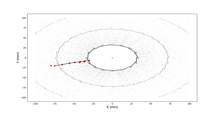

An ANN bucket of 20 hits (red points) and the largest particle represented by the line. Transverse view of the TrackML detector.

Yes, indeed the full electron trace was contained in this bucket. Was this a lucky scenario? What is the average particle size we actually get when querying 20 neighbors? Let’s look at the distribution of the largest particle size in all possible ANN queries.

We can do this by simply storing the largest count in every query similarly to what we did visualy with the electron bucket. Using the most_common() function on the Counter allows to return only the id and size of the largest particle. This function takes approximately 40 seconds since the number of hits is quite large and Counter() is not the fastest option (but it is the nicest).

largest_particle_size=[]
for i in data.index.values:
   bucket_idx=annoy_idx.get_nns_by_item(i,Nb_neighbors)
   c=Counter(data.iloc[bucket_idx].particle_id).most_common(1)[0][1]         
   largest_particle_size.append(c)

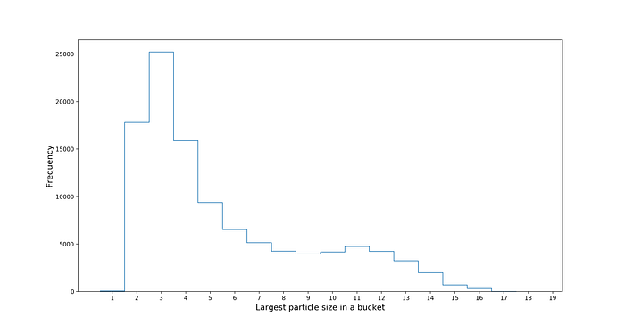
It turns out that getting a 16 hit particle in 20 hit ANN bucket was somewhat lucky. The are less than 1K queries containing such a high number of same-particle hits. The majority of ANN buckets contain 3, 2 and 4 hits particle traces. If however we try increasing the number neighbors queried from 20 to … 50, the distribution shifts!

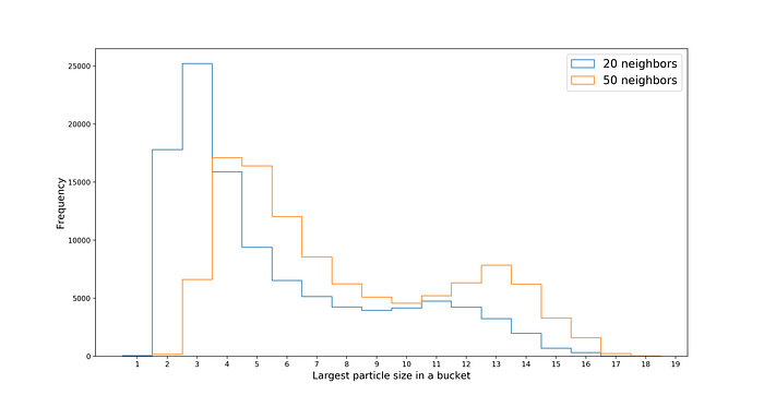
Now the majority of buckets contain 4 and 5 hits produced by the same particle. The overal distribution nicely shifts towards the right allowing to contain larger traces.

Making 10K (approximately the number of particles in an event) queries of 50 hits takes 400ms using the Annoy librabry. Can we optimize further the ANN queries to contain only large traces of particles?

So far, we only explored ANN buckets built with an angular distance. Is there a better choice ? Stay tuned for the next post!

The complete code can be found on github.com/greysab/pyhep